Statistics: Lord’s Resistance Army - Uganda

BACKGROUND

The data are from Chirstopher Blattman and J Annan. 2010. “The consequences of child soldiering” Review of Economics and Statistics 92 (4):882-898

The data are from a panel survey of male youth in war-afflicted regions of Uganda. The authors want to estimate the impact of forced military service on various outcomes. They focus on Uganda because there were a significant number of abductions of young men into Lord’s Resistance Army. Blattman and Annan describe the abductions as follows:

Abduction was large-scale and seemingly indiscriminate; 60,000 to 80,000 youth are estimated to have been abducted and more than a quarter of males currently aged 14 to 30 in our study region were abducted for at least two weeks. Most were abducted after 1996 and from one of the Acholi districts of Gulu, Kitgum, and Pader.

Youth were typically taken by roving groups of 10 to 20 rebels during night raids on rural homes. Adolescent males appear to have been the most pliable, reliable and effective forced recruits, and so were disproportionately targeted by the LRA. Youth under age 11 and over 24 tended to be avoided and had a high probability of immediate release. Lengths of abduction ranged from a day to ten years, averaging 8.9 months in our sample. Youth who failed toe escape were trained as fighters and, after a few months, received a gun. Two thirds of abductees were forced to perpetrate a crime or violence. A third eventually became fighters and a fifth were forced to murder soldiers, civilians, or even family members in order to bind them to the group, to reduce their fear of killing, and to discourage disobedience.

ANALYSIS

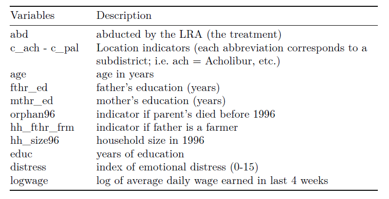
In this problem we will look at the effect of abduction on educ (years of education).The abd variable is the treatment in this case. Note that educ, distress, and logwage are all outcomes/post-treatment variables.

When using linear regression model to calculate the naive average treatment effect (ATE) of abduction on education, the coefficient was -.60, meaning that if someone is abducted, he would have about 0.6 less years of education than those that are not abducted. Standard error of this estimate is 2.88.

Would it be the same case when using the propensity score matching method?

Propensity Score Matching

Logit Regression Model

#Formular to use in logit model
blattman.formu <- abd ~ C_ach + C_akw + C_ata + C_kma + C_oro + C_pad + C_paj + age + fthr_ed + mthr_ed + orphan96 + hh_fthr_frm + hh_size96

#Logit regression model
glm1 <- glm(blattman.formu, family = binomial, data = blattman)

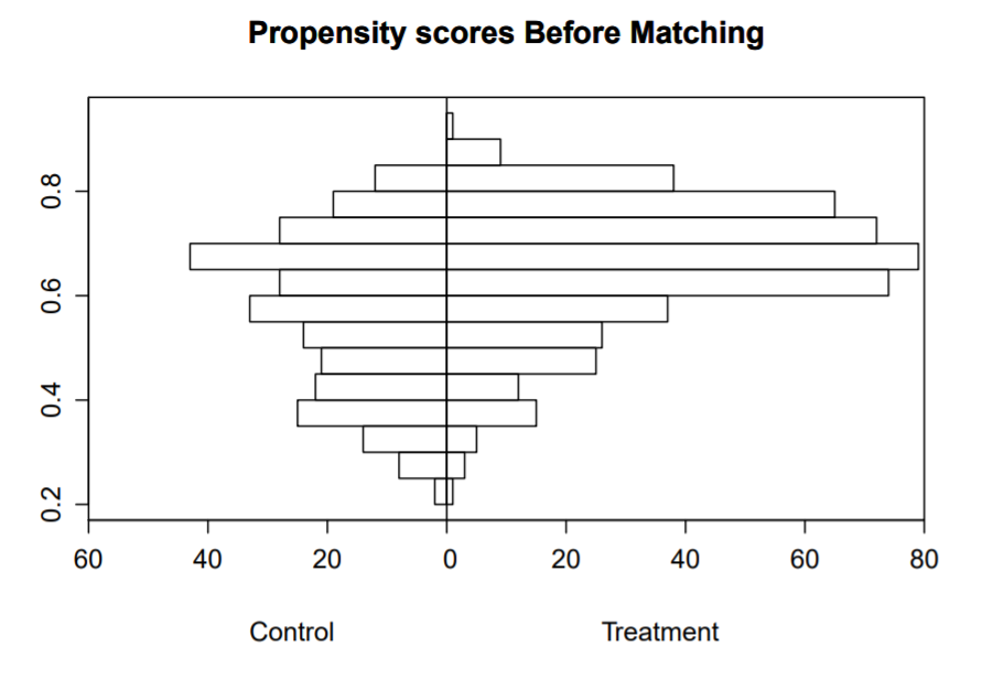
Plot Propensity scores before matching

#Assign calculated propensity score to each observation
blattman$psvalue <- predict(glm1, type="response")

#Propensity score before matching
histbackback(split(blattman$psvalue, blattman$abd), main="Propensity scores Before Matching",xlab=c('Control','Treatment'))

Divide the data into 6 equally-sized strata On average, each stratum (subset) will contain 124 observations.

blattman$cut2 <- cut2(blattman$psvalue, g=6, levels.mean = T)

blattman$cut1 <- cut(as.numeric(blattman$cut2), 6, m=124, labels = F)

Linear regression to calculate the ATE for each stratum individually

##Group 1
reg.group1<-lm(educ~abd + C_ach + C_akw + C_ata + C_kma + C_oro + C_pad + C_paj + age + fthr_ed + mthr_ed + orphan96 + hh_fthr_frm + hh_size96,data=blattman, subset = (cut1 == 1))

Apply the same code for the rest of the strata.

Linear regression to calculate the overall ATE

reg.1<-lm(educ~abd + C_ach + C_akw + C_ata + C_kma + C_oro + C_pad + C_paj + age + fthr_ed + mthr_ed + orphan96 + hh_fthr_frm + hh_size96,data=blattman)

Output Summary

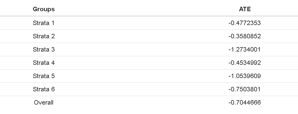
Overall, the ATE of being abducted was about 0.7 years of less education on average compared to those who were not abducted.

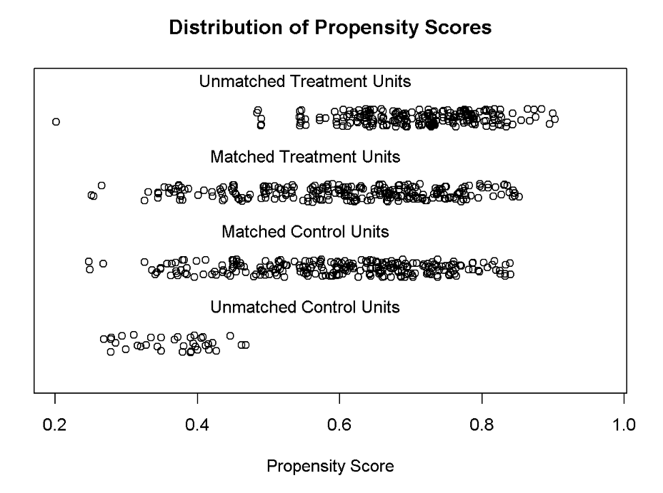
Distribution of propensity scores using a nearest neighbor match

m.nn <- matchit(blattman.formu, data = blattman, caliper = .1, method = 'nearest')

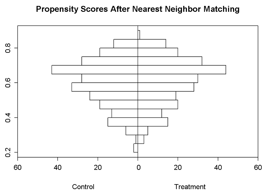
Back-to-back Histogram to compare groups after PSM

nn.match <- match.data(m.nn)

histbackback(split(nn.match$psvalue, nn.match$abd),
             main = "Propensity Scores After Nearest Neighbor Matching",
             xlab = c("Control", "Treatment"))

Test for balance

#Unconditional
xBalance(blattman.formu, data = blattman, report=c("chisquare.test"))

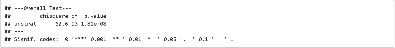
Balance before matching gives a chi-square statistic that we reject null, and say that the means are not the same. (we want the means to be similar).

#Nearest neighbor
xBalance(blattman.formu, data = as.data.frame(nn.match), report = 'chisquare.test')

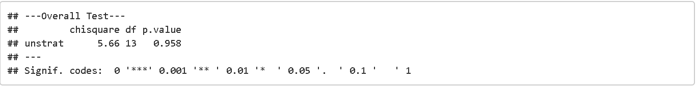
Balance after matching yields a chi-square statistic which we fail to reject. So this means the means of the two groups are similar, which is what we want.

ATE using nearest neighbors with and without covariates

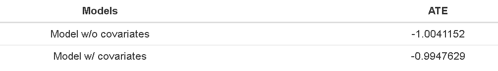
The average treatment effect does not change much from the model without covariates to the model including them. This indicates that the matching did eliminate a lot of the omitted variable bias.

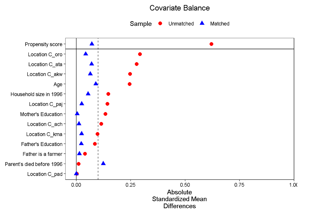
Use the cobalt package to make a “Love plot”